Irrigation module
Overview
This module estimates the electricity requirements to pump ground- and surface-water for crop irrigation. The model simulates in a simple yet scientifically sound manner the link between crop distribution, water use and electricity demand. The model is sufficiently flexible to incorporate potential changes in harvested area, climate, irrigation technologies and water management constraints. The methodology consists of three main phases, set out in the bullets below and summarised in Figure below.
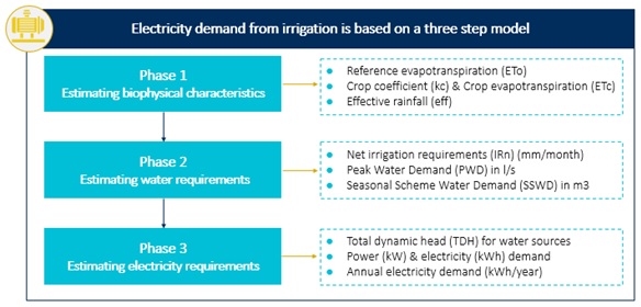
Methodological steps of the of irrigation model
Phase 1 models the agricultural calendar and the corresponding planting, growing and harvesting seasons for crops grown in the study area, as determined by input geospatial data. Temporal and spatial criteria regarding the crop water needs in the various climate zones and land conditions are taken into consideration.
Phase 2 models the reference (ET0) and crop (ETc) evapotranspiration in each of the modelling months. Water requirements are then estimated as the difference between ETc and effective rainfall in a given location.
Phase 3 estimates the electricity (kWh) necessary to supply the required water in each location. The assessment of electricity requirements depend on the morphology of the land, both underground and over ground, and take into account the different operating and application pressure levels required under different irrigation techniques and technologies.
Input data preparation
Input 1: Crop calendar that describes the crop phases (or cycles) within a calendat year. Note that this may vary per crop and region. That is, the modeler can specify different crop cycles per AoI (e.g. admininstrative level) if this information is available. An example of such a file is available in the project’s repository as Sample_Maize_Crop_Calendar for rainfed maize in Mozambique.
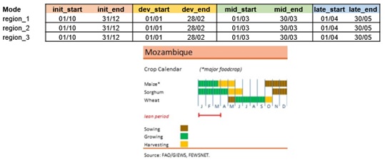
Sample crop calendar for rainfed maize in Mozambique
Input 2: Crop layer where each location represents a potential demand node for irrigation (e.g. farm). The resolution (spatial & temporal) may vary and it depends on data availability for the AOI. Once collected, the crop layer shall be transformed into a vector dataset (in csv format) that contains the following attributes:
- country (name)
- state (name - admin 1 or 2)
- lat, lon (deg)
- crop (name - modelling crop)
- Fraction (%)
- harv_area (harvested area in ha)
- curr_yield (Current yield in kg/ha)
- max_yield (Maximun yield in kg/ha)
- gw_depth (Ground water depth in m)
- sw_dist (Distance to surface water in m)
- sw_depth (surface water depth in m)
- elevation (in m)
- awsc (Water storage capacity of the soil in mm/m)
- sw_suit_idx (Surface irrigation suitability index: 1= suitable 9999= non suitable)
- prec_i (Average precipitation in mm/month; i=1-12)
- srad_i (Average solar irradiation per month in kJ m-2 day-1; i=1-12)
- wind_i (Average wind speed per month in m s-1; i=1-12)
- tavg_i, tmax_i, tmin_i(Average, Max, Min temperature per month in C; i=1-12)
An example of such a file is available in the project’s repository as Sample_Moz_Maize_1km.
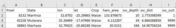
Sample of crop input data showing the supporting columns with attributes
Note
- Features related to surface water (sw_dist, sw_depth, sw_suit_idx) can be extracted with the used of this QGIS plugin. It was developed by the team and together with instructions for installation and use.
- Extraction of other features can be done using the open source script Agrodem_Prepping, which is based on spatial packages and Qgis.
Parameterization & model run
Once the crop calendar information is collected and the crop vector layer fully attributed, the irrigation model is ready to run. Note that this is available in the project’s repository as agrodem.
Note that there are a few input parameters that need to be determined in the model per se. These include:
- Kc factor for init. – dev/mid – late crop cycles (source FAO )
- Current yield of the crop (in kg/ha)
- Maximum yield of the crop (in kg/ha)
- Effective Rooting Depth (in meters)
- Field Application Efficiency – aeff (%)
- Distribution Efficiency – deff (%)
- Pumping hours per day (in hours)
- Pressure head (in meters)
- Powered pump efficiency – electric (%)
- Motor efficiency (%)
Note
These values are available in the literature. However, they are predominantly based on value-laden judgements and assumptions of the modeller, informed - in best case scenario – in consultation with agriculture experts.
Output data
The output of the model indicates electricity requirements for irrigation of the selected crop and AoI. The spatial resolution of the results are defined by the initial vector later and stored in .csv format. Each row indicates a particular location (e.g. farm); and each column indicates a particular attribute for this location. These include all attributes used to derive electricity requirement in the first place and products of the analysis (water and electricity requirements).
Results are available in any GIS compatible, OGC complaint format (e.g .shp, .csv, .gpkg, .tiff). We have selected the .csv format as it can provide information in tabular form but also be visualized in relatively easy and straight-forward manner in a GIS environment.
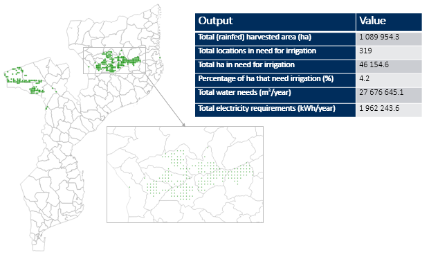
Indicative results indicating locations of rainfed maize in need for irrigation in the base year (2017-18) in Mozambique
Note
The final result file includes only the locations with non-zero electricity requirement. This is to reduce volume of output data. One might select to extract the full list of locations by minor modifications in the code base, if interested in all products of the analysis.
Special notes
The irrigation model elaborates on three major steps that assess electricity requirements for irrigation (surface or ground) for an AOI. It can receive crop allocation data at varying temporal and spatial resolution and is modular, thus fully customizable as per need.
However,
- Level of parameterization is high and highly dependent on experts’ value-laden judgement. That is, model input parameters should be decided with caution and under the consultation of local agriculture/energy experts.
- The model can be used for a quick, screening analysis however one should be aware that many assumptions were set in place. For example, the model assumes that water reservoirs (both surface and underground) have unlimited flow capacity for irrigation purposes. In reality limits do exist – these are usually covered in detailed hydrological models/analyses – yet not part of this analysis.
- Spatial resolution of input data may have an impact on the results. Low resolution is bound to rough assumptions; whereas higher resolution can leverage spatial information with higher accuracy – and thus the insights one can get out of this exercise. This part is (partially) covered in the next section.